Model Training
Oracle AutoML
Oracle AutoML automates the machine learning experience. It replaces the laborious and time consuming tasks of the data scientist whose workflow is as follows:
Select a model from a large number of viable candidate models.
For each model, tune the hyperparameters.
Select only predictive features to speed up the pipeline and reduce over fitting.
Ensure the model performs well on unseen data (also called generalization).

Oracle AutoML automates this workflow and provides you with an optimal model given a time budget. In addition to incorporating these typical machine learning workflow steps, Oracle AutoML is also optimized to produce a high quality model very efficiently. You can achieve this with the following:
Scalable design: All stages in the Oracle AutoML pipeline exploit both internode and intranode parallelism, which improves scalability and reduces runtime.
Intelligent choices reduce trials in each stage: Algorithms and parameters are chosen based on dataset characteristics. This ensures that the selected model is accurate and is efficiently selected. You can achieve this using meta learning throughout the pipeline. Meta learning is used in:
Algorithm selection to choose an optimal model class.
Adaptive sampling to identify the optimal set of samples.
Feature selection to determine the ideal feature subset.
Hyperparameter optimization.
The following topics detail the Oracle AutoML pipeline and individual stages of the pipeline:
Keras
Keras is an open source neural network library. It can run on top of TensorFlow, Theano, and Microsoft Cognitive Toolkit. By default, Keras uses TensorFlow as the backend. Keras is written in Python, but it has support for R and PlaidML, see About Keras.
These examples examine a binary classification problem predicting churn. This is a common type of problem that can be solved using Keras, Tensorflow, and scikit-learn.
If the data is not cached, it is pulled from github, cached, and then loaded.
from os import path
import numpy as np
import pandas as pd
import requests

import logging
logging.basicConfig(format='%(levelname)s:%(message)s', level=logging.ERROR)

churn_data_file = '/tmp/churn.csv'
if not path.exists(churn_data_file):
    # fetch sand save some data
    print('fetching data from web...', end =" ")
    r = requests.get('oci://hosted-ds-datasets@hosted-ds-datasets/churn/dataset.csv')
    with open(churn_data_file, 'wb') as fd:
        fd.write(r.content)
    print("Done")

df = pd.read_csv(churn_data_file)
Keras needs to be imported and scikit-learn needs to be imported to generate metrics. Most of the data preprocessing and modeling can be done using the ADS library. However, the following example demonstrates how to do
these tasks with external libraries:
from keras.layers import Dense
from keras.models import Sequential
from sklearn.metrics import confusion_matrix, roc_auc_score
from sklearn.model_selection import train_test_split
from sklearn.preprocessing import LabelEncoder, OneHotEncoder
from sklearn.preprocessing import StandardScaler
The first step is data preparation. From the pandas.DataFrame, you extract the X and Y-values as numpy arrays. The feature selection is performed manually. The next step is feature encoding using sklearn LabelEncoder. This converts categorical variables into ordinal values (‘red’, ‘green’, ‘blue’ –> 0, 1, 2) to be compatible with Keras. The data is then split using a 80/20 ratio. The training is performed on 80% of the data. Model testing is performed on the remaining 20% of the data to evaluate how well the model generalizes.
feature_name = ['CreditScore', 'Geography', 'Gender', 'Age', 'Tenure', 'Balance',
                'NumOfProducts', 'HasCrCard', 'IsActiveMember', 'EstimatedSalary']

response_name = ['Exited']
data = df[[val for sublist in [feature_name, response_name] for val in sublist]].copy()

# Encode the category columns
for col in ['Geography', 'Gender']:
  data.loc[:, col] = LabelEncoder().fit_transform(data.loc[:, col])

# Do an 80/20 split for the training and test data
train, test = train_test_split(data, test_size=0.2, random_state=42)

# Scale the features and split the features away from the response
sc = StandardScaler() # Feature Scaling
X_train = sc.fit_transform(train.drop('Exited', axis=1).to_numpy())
X_test = sc.transform(test.drop('Exited', axis=1).to_numpy())
y_train = train.loc[:, 'Exited'].to_numpy()
y_test = test.loc[:, 'Exited'].to_numpy()
The following shows the neural network architecture. It is a sequential model with an input layer with 10 nodes. It has two hidden layers with 255 densely connected nodes and the ReLu activation function. The output layer has a single node with a sigmoid activation function because the model is doing binary classification. The optimizer is Adam and the loss function is binary cross-entropy. The model is optimized on the accuracy metric. This takes several minutes to run.
keras_classifier = Sequential()
keras_classifier.add(Dense(units=1, kernel_initializer='uniform', activation='sigmoid'))
keras_classifier.add(Dense(units=255, kernel_initializer='uniform', activation='relu'))
keras_classifier.add(Dense(units=255, kernel_initializer='uniform', activation='relu', input_dim=10))
keras_classifier.compile(optimizer='adam', loss='binary_crossentropy', metrics=['accuracy'])
keras_classifier.fit(X_train, y_train, batch_size=10, epochs=25)
To evaluate this model, you could use sklearn or ADS.
This example uses sklearn:
y_pred = keras_classifier.predict(X_test)
y_pred = (y_pred > 0.5)

cm = confusion_matrix(y_test, y_pred)
auc = roc_auc_score(y_test, y_pred)

print("confusion_matrix:\n", cm)
print("roc_auc_score", auc)
This example uses the ADS evaluator package:
from ads.common.data import MLData
from ads.common.model import ADSModel
from ads.evaluations.evaluator import ADSEvaluator

eval_test = MLData.build(X = pd.DataFrame(sc.transform(test.drop('Exited', axis=1)), columns=feature_name),
                         y = pd.Series(test.loc[:, 'Exited']),
                         name = 'Test Data')
eval_train = MLData.build(X = pd.DataFrame(sc.transform(train.drop('Exited', axis=1)), columns=feature_name),
                          y = pd.Series(train.loc[:, 'Exited']),
                          name = 'Training Data')
clf = ADSModel.from_estimator(keras_classifier, name="Keras")
evaluator = ADSEvaluator(eval_test, models=[clf], training_data=eval_train)
Scikit-Learn
The sklearn pipeline can be used to build a model on the same churn dataset that was used in the Keras section. The pipeline allows the model to contain multiple stages and transformations. Typically, there are pipeline stages for feature encoding, scaling, and so on. In this pipeline example, a LogisticRegression estimator is used:
from sklearn.linear_model import LogisticRegression
from sklearn.pipeline import Pipeline

pipeline_classifier = Pipeline(steps=[
  ('clf', LogisticRegression())
])

pipeline_classifier.fit(X_train, y_train)
You can evaluate this model using sklearn or ADS.
XGBoost
XGBoost is an optimized, distributed gradient boosting library designed to be efficient, flexible, and portable. It implements machine learning algorithms under the Gradient Boosting framework. XGBoost provides parallel tree boosting (also known as Gradient Boosting Decision Tree, Gradient Boosting Machines [GBM]) and can be used to solve a variety of data science applications. The unmodified code runs on several distributed environments (Hadoop, SGE, andMPI) and can processes billions of observations, see the XGBoost Documentation.
Import XGBoost with:
from xgboost import XGBClassifier

xgb_classifier = XGBClassifier(nthread=1)
xgb_classifier.fit(eval_train.X, eval_train.y)
From the three estimators, we create three ADSModel objects. A Keras classifier, a sklearn pipeline with a single LogisticRegression stage, and an XGBoost model:
from ads.common.model import ADSModel
from ads.evaluations.evaluator import ADSEvaluator
from ads.common.data import MLDataa

keras_model = ADSModel.from_estimator(keras_classifier)
lr_model = ADSModel.from_estimator(lr_classifier)
xgb_model = ADSModel.from_estimator(xgb_classifier)

evaluator = ADSEvaluator(eval_test, models=[keras_model, lr_model, xgb_model], training_data=eval_train)
evaluator.show_in_notebook()
ADSTuner
In addition to the other services for training models, ADS includes a hyperparameter tuning framework called ADSTuner.
ADSTuner supports using several hyperparameter search strategies that plug into common model architectures like sklearn.
ADSTuner further supports users defining their own search spaces and strategies. This makes ADSTuner functional and useful with any ML library that doesn’t include hyperparameter tuning.
First, import the packages:
import category_encoders as ce
import lightgbm
import logging
import numpy as np
import os
import pandas as pd
import pytest
import sklearn
import xgboost

from ads.hpo.distributions import *
from ads.hpo.search_cv import ADSTuner, NotResumableError
from ads.hpo.stopping_criterion import *
from lightgbm import LGBMClassifier
from sklearn import preprocessing
from sklearn.compose import ColumnTransformer
from sklearn.datasets import load_iris, load_boston
from sklearn.decomposition import PCA
from sklearn.ensemble import AdaBoostRegressor, AdaBoostClassifier
from sklearn.feature_selection import SelectKBest, f_classif
from sklearn.impute import SimpleImputer
from sklearn.linear_model import SGDClassifier, LogisticRegression
from sklearn.metrics import make_scorer, f1_score
from sklearn.model_selection import train_test_split
from sklearn.pipeline import Pipeline
from sklearn.preprocessing import StandardScaler
from xgboost import XGBClassifier
This is an example of running the ADSTuner on a support model SGD from sklearn:
model = SGDClassifier() ##Initialize the model
X, y = load_iris(return_X_y=True)
X_train, X_valid, y_train, y_valid = train_test_split(X, y)
tuner = ADSTuner(model, cv=3) ## cv is cross validation splits
tuner.search_space() ##This is the default search space
tuner.tune(X_train, y_train, exit_criterion=[NTrials(10)])
ADSTuner generates a tuning report that lists its trials, best performing hyperparameters, and performance statistics with:
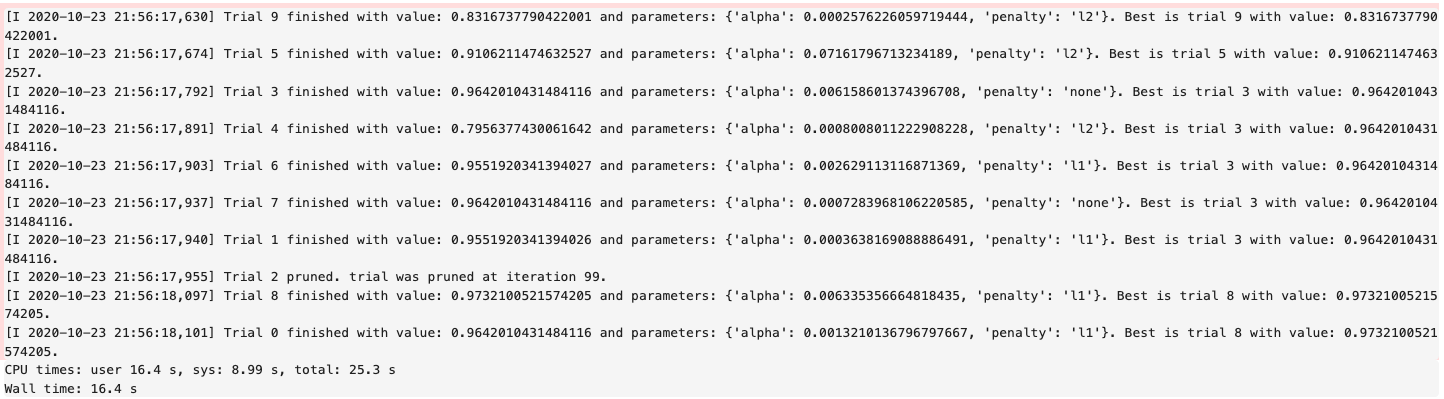
You can use tuner.best_score to get the best score on the scoring metric used (accessible as``tuner.scoring_name``)
The best selected parameters are obtained with tuner.best_params and the complete record of trials with tuner.trials
If you have further compute resources and want to continue hyperparameter optimization on a model that has already been optimized, you can use:
tuner.resume(exit_criterion=[TimeBudget(5)], loglevel=logging.NOTSET)
print('So far the best {} score is {}'.format(tuner.scoring_name, tuner.best_score))
print("The best trial found was number: " + str(tuner.best_index))
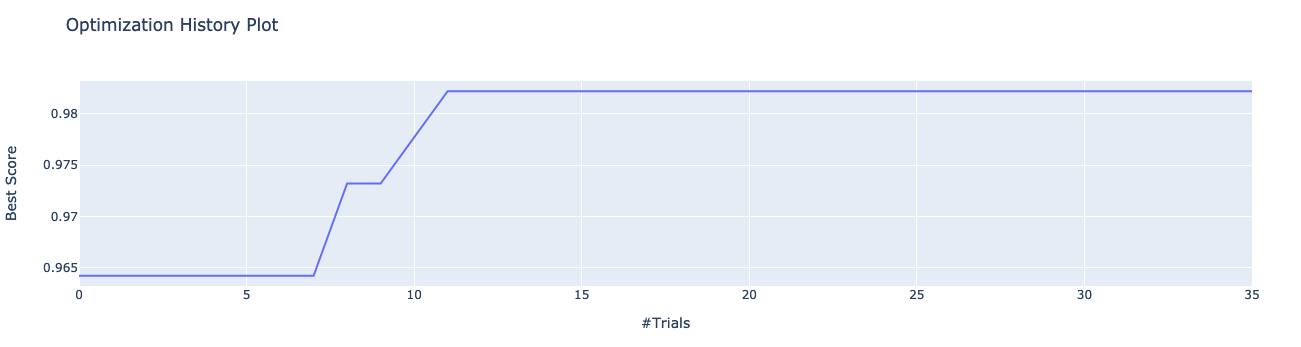
ADSTuner has some robust visualization and plotting capabilities:
tuner.plot_best_scores()
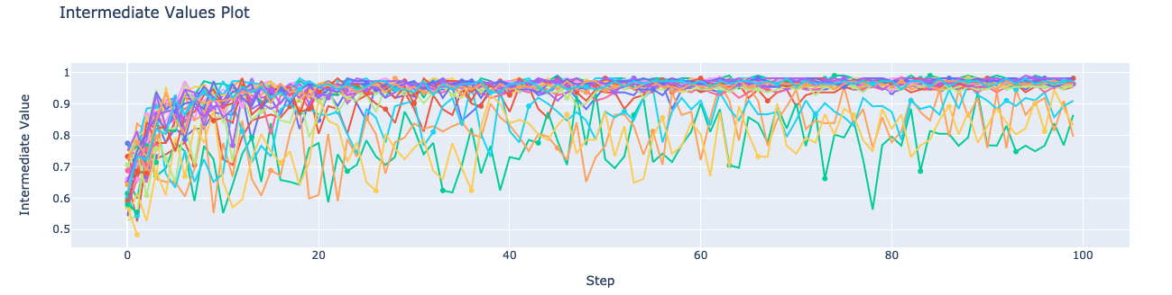
tuner.plot_intermediate_scores()
tuner.search_space()
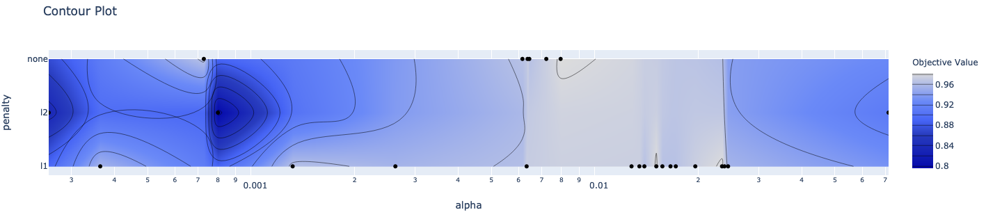
tuner.plot_contour_scores(params=['penalty', 'alpha'])
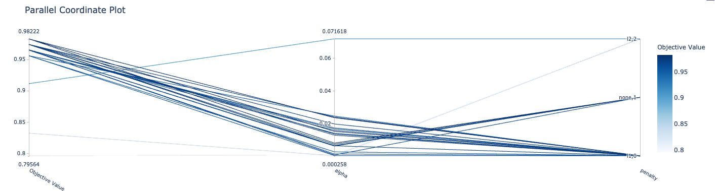
tuner.plot_parallel_coordinate_scores(params=['penalty', 'alpha'])
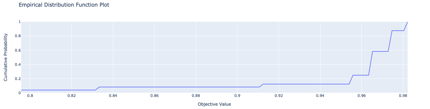
tuner.plot_edf_scores()
These commands produce the following plots:
ADSTuner supports custom scoring functions and custom search spaces. This example uses a different model:
model2 = LogisticRegression()
tuner = ADSTuner(model2,
                 strategy = {
                 'C': LogUniformDistribution(low=1e-05, high=1),
                 'solver': CategoricalDistribution(['saga']),
                 'max_iter': IntUniformDistribution(500, 1000, 50)},
                 scoring=make_scorer(f1_score, average='weighted'),
                 cv=3)
tuner.tune(X_train, y_train, exit_criterion=[NTrials(5)])
ADSTuner doesn’t support every model. The supported models are:
‘Ridge’,
‘RidgeClassifier’,
‘Lasso’,
‘ElasticNet’,
‘LogisticRegression’,
‘SVC’,
‘SVR’,
‘LinearSVC’,
‘LinearSVR’,
‘DecisionTreeClassifier’,
‘DecisionTreeRegressor’,
‘RandomForestClassifier’,
‘RandomForestRegressor’,
‘GradientBoostingClassifier’,
‘GradientBoostingRegressor’,
‘XGBClassifier’,
‘XGBRegressor’,
‘ExtraTreesClassifier’,
‘ExtraTreesRegressor’,
‘LGBMClassifier’,
‘LGBMRegressor’,
‘SGDClassifier’,
‘SGDRegressor’
The AdaBoostRegressor model is not supported. This is an example of a custom strategy to use with this model:
model3 = AdaBoostRegressor()
X, y = load_boston(return_X_y=True)
X_train, X_valid, y_train, y_valid = train_test_split(X, y)
tuner = ADSTuner(model3, strategy={'n_estimators': IntUniformDistribution(50, 100)})
tuner.tune(X_train, y_train, exit_criterion=[TimeBudget(5)])
Finally, ADSTuner supports sklearn pipelines:
df, target = pd.read_csv(os.path.join('~', 'advanced-ds', 'tests', 'vor_datasets', 'vor_titanic.csv')), 'Survived'
X = df.drop(target, axis=1)
y = df[target]

numeric_features = X.select_dtypes(include=['int64', 'float64', 'int32', 'float32']).columns
categorical_features = X.select_dtypes(include=['object', 'category', 'bool']).columns

y = preprocessing.LabelEncoder().fit_transform(y)

X_train, X_valid, y_train, y_valid = train_test_split(X, y, test_size=0.3, random_state=42)

num_features = len(numeric_features) + len(categorical_features)

numeric_transformer = Pipeline(steps=[
    ('num_imputer', SimpleImputer(strategy='median')),
    ('num_scaler', StandardScaler())
])

categorical_transformer = Pipeline(steps=[
    ('cat_imputer', SimpleImputer(strategy='constant', fill_value='missing')),
    ('cat_encoder', ce.woe.WOEEncoder())
])

preprocessor = ColumnTransformer(
    transformers=[
        ('num', numeric_transformer, numeric_features),
        ('cat', categorical_transformer, categorical_features)
    ]
)

pipe = Pipeline(
    steps=[
        ('preprocessor', preprocessor),
        ('feature_selection', SelectKBest(f_classif, k=int(0.9 * num_features))),
        ('classifier', LogisticRegression())
    ]
)

def customerize_score(y_true, y_pred, sample_weight=None):
    score = y_true == y_pred
    return np.average(score, weights=sample_weight)

score = make_scorer(customerize_score)
ads_search = ADSTuner(
    pipe,
    scoring=score,
    strategy='detailed',
    cv=2,
    random_state=42
)
ads_search.tune(X=X_train, y=y_train, exit_criterion=[NTrials(20)])
Example
A hyperparameter is a parameter that is used to control a learning process. This is in contrast to other parameters that are learned in the training process. The process of hyperparameter optimization is to search for hyperparameter values by building many models and assessing their quality. This notebook provides an overview of the ADSTuner hyperparameter optimization engine. ADSTuner can optimize any estimator object that follows the scikit-learn API.
import category_encoders as ce
import lightgbm
import logging
import numpy as np
import os
import pandas as pd
import sklearn
import time

from ads.hpo.stopping_criterion import *
from ads.hpo.distributions import *
from ads.hpo.search_cv import ADSTuner, State

from sklearn import preprocessing
from sklearn.compose import ColumnTransformer
from sklearn.datasets import load_iris, load_boston
from sklearn.decomposition import PCA
from sklearn.impute import SimpleImputer
from sklearn.linear_model import SGDClassifier, LogisticRegression
from sklearn.metrics import make_scorer, f1_score
from sklearn.model_selection import train_test_split
from sklearn.pipeline import Pipeline
from sklearn.preprocessing import StandardScaler
from sklearn.feature_selection import SelectKBest, f_classif
Introduction
Hyperparameter optimization requires a model, dataset, and an ADSTuner object to perform the search.
ADSTuner() Performs a hyperparameter search using cross-validation. You can specify the number of folds you want to use with the cv parameter.
The ADSTuner() needs a search space to tune the hyperparameters in so you use the strategy parameter. This parameter can be set in two ways. You can specify detailed search criteria or you can use the built-in defaults. For the supported model classes, ADSTuner provides perfunctoryand detailed search spaces that are optimized for the class of model that is being used. The perfunctory option is optimized for a small search space so that the most important hyperparameters are tuned. Generally, this option is used early in your search as it reduces the computational cost and allows you to assess the quality of the model class that you are using. The detailed search space instructs ADSTuner to cover a broad search space by tuning more hyperparameters. Typically, you would use it when you have determined what class of model is best suited for the dataset and type of problem you are working on. If you have experience with the dataset and have a good idea of what the best hyperparameter values are, you can explicitly specify the search space. You pass a dictionary that defines the search space into the strategy.
The parameter storage takes a database URL. For example, sqlite:////home/datascience/example.db. When storage is set to the default value None, a new sqlite database file is created internally in the tmp folder with a unique name. The name format is sqlite:////tmp/hpo_*.db. study_name is the name of this study for this ADSTuner object. One ADSTuner object only has one study_name. However, one database file can be shared among different ADSTuner objects. load_if_exists controls whether to load an existing study from an existing database file. If False, it raises a DuplicatedStudyError when the study_name exists.
The loglevel parameter controls the amount of logging information displayed in the notebook.
This notebook uses the scikit-learn SGDClassifer() model and the iris dataset. This model object is a regularized linear model with stochastic gradient descent (SGD) used to optimize the model parameters.
The next cell creates the SGDClassifer() model, initialize an ADSTuner object, and loads the iris data.
tuner = ADSTuner(SGDClassifier(), cv=3, loglevel=logging.WARNING)
X, y = load_iris(return_X_y=True)
A new study created with name: hpo_22cfd4d5-c512-4e84-b7f8-d6d9c721ff05
Each model class has a set of hyperparameters that you need to optimized. The strategy attribute returns what strategy is being used. This can be perfunctory, detailed, or a dictionary that defines the strategy. The method search_space() always returns a dictionary of hyperparameters that are to be searched. Any hyperparameter that is required by the model, but is not listed, uses the default value that is defined by the model class. To see what search space is being used for your model class when strategy is perfunctory or detailed use the search_space() method to see the details.
The adstuner_search_space_update.ipynb notebook has detailed examples about how to work with and update the search space.
The following code snippet shows the search strategy and the search space.
print(f'Search Space for strategy "{tuner.strategy}" is: \n {tuner.search_space()}')
Search Space for strategy "perfunctory" is:
 {'alpha': LogUniformDistribution(low=0.0001, high=0.1), 'penalty': CategoricalDistribution(choices=['l1', 'l2', 'none'])}
The tune() method starts a tuning process. It has a synchronous and asynchronous mode for tuning. The mode is set with the synchronous parameter. When it is set to False, the tuning process runs asynchronously so it runs in the background and allows you to continue your work in the notebook. When synchronous is set to True, the notebook is blocked until tune() finishes running. The adntuner_sync_and_async.ipynb notebook illustrates this feature in a more detailed way.
The ADSTuner object needs to know when to stop tuning. The exit_criterion parameter accepts a list of criteria that cause the tuning to finish. If any of the criteria are met, then the tuning process stops. Valid exit criteria are:
NTrials(n): Run fornnumber of trials.ScoreValue(s): Run until the score value exceedss.TimeBudget(t): Run fortseconds.
The default behavior is to run for 50 trials (NTrials(50)).
The stopping criteria are listed in the ads.hpo.stopping_criterion module.
Synchronous Tuning
This section demonstrates how to perform a synchronous tuning process with the exit criteria based on the number of trials. In the next cell, the synchronous parameter is set to True and the exit_criterion is set to [NTrials(5)].
tuner.tune(X, y, exit_criterion=[NTrials(5)], synchronous=True)
You can access a summary of the trials by looking at the various attributes of the tuner object. The scoring_name attribute is a string that defines the name of the scoring metric. The best_score attribute gives the best score of all the completed trials. The best_params parameter defines the values of the hyperparameters that have to lead to the best score. Hyperparameters that are not in the search criteria are not reported.
print(f"So far the best {tuner.scoring_name} score is {tuner.best_score} and the best hyperparameters are {tuner.best_params}")
So far the best mean accuracy score is 0.9666666666666667 and the best hyperparameters are {'alpha': 0.002623793623610696, 'penalty': 'none'}
You can also look at the detailed table of all the trials attempted:
tuner.trials.tail()
| number | value | datetime_start | datetime_complete | duration | params_alpha | params_penalty | user_attrs_mean_fit_time | user_attrs_mean_score_time | user_attrs_mean_test_score | user_attrs_metric | user_attrs_split0_test_score | user_attrs_split1_test_score | user_attrs_split2_test_score | user_attrs_std_fit_time | user_attrs_std_score_time | user_attrs_std_test_score | state | |
|---|---|---|---|---|---|---|---|---|---|---|---|---|---|---|---|---|---|---|
| 0 | 0 | 0.966667 | 2021-04-21 20:04:03.582801 | 2021-04-21 20:04:05.276723 | 0 days 00:00:01.693922 | 0.002624 | none | 0.172770 | 0.027071 | 0.966667 | mean accuracy | 1.00 | 0.94 | 0.96 | 0.010170 | 0.001864 | 0.024944 | COMPLETE |
| 1 | 1 | 0.760000 | 2021-04-21 20:04:05.283922 | 2021-04-21 20:04:06.968774 | 0 days 00:00:01.684852 | 0.079668 | l2 | 0.173505 | 0.026656 | 0.760000 | mean accuracy | 0.70 | 0.86 | 0.72 | 0.005557 | 0.001518 | 0.071181 | COMPLETE |
| 2 | 2 | 0.960000 | 2021-04-21 20:04:06.977150 | 2021-04-21 20:04:08.808149 | 0 days 00:00:01.830999 | 0.017068 | l1 | 0.185423 | 0.028592 | 0.960000 | mean accuracy | 1.00 | 0.92 | 0.96 | 0.005661 | 0.000807 | 0.032660 | COMPLETE |
| 3 | 3 | 0.853333 | 2021-04-21 20:04:08.816561 | 2021-04-21 20:04:10.824708 | 0 days 00:00:02.008147 | 0.000168 | l2 | 0.199904 | 0.033303 | 0.853333 | mean accuracy | 0.74 | 0.94 | 0.88 | 0.005677 | 0.001050 | 0.083799 | COMPLETE |
| 4 | 4 | 0.826667 | 2021-04-21 20:04:10.833650 | 2021-04-21 20:04:12.601027 | 0 days 00:00:01.767377 | 0.001671 | l2 | 0.180534 | 0.028627 | 0.826667 | mean accuracy | 0.80 | 0.96 | 0.72 | 0.009659 | 0.002508 | 0.099778 | COMPLETE |
Asynchronously Tuning
ADSTuner() tuner can be run in an asynchronous mode by setting synchronous=False in the tune() method. This allows you to run other Python commands while the tuning process is executing in the background. This section demonstrates how to run an asynchronous search for the optimal hyperparameters. It uses a stopping criteria of five seconds. This is controlled by the parameter exit_criterion=[TimeBudget(5)].
The next cell starts an asynchronous tuning process. A loop is created that prints the best search results that have been detected so far by using the best_score attribute. It also displays the remaining time in the time budget by using the time_remaining attribute. The attribute status is used to exit the loop.
# This cell will return right away since it's running asynchronous.
tuner.tune(exit_criterion=[TimeBudget(5)])
while tuner.status == State.RUNNING:
    print(f"So far the best score is {tuner.best_score} and the time left is {tuner.time_remaining}")
    time.sleep(1)
So far the best score is 0.9666666666666667 and the time left is 4.977275848388672
So far the best score is 0.9666666666666667 and the time left is 3.9661824703216553
So far the best score is 0.9666666666666667 and the time left is 2.9267797470092773
So far the best score is 0.9666666666666667 and the time left is 1.912914752960205
So far the best score is 0.9733333333333333 and the time left is 0.9021461009979248
So far the best score is 0.9733333333333333 and the time left is 0
The attribute best_index gives you the index in the trials data frame where the best model is located.
tuner.trials.loc[tuner.best_index, :]
number                                                  10
value                                                 0.98
datetime_start                  2021-04-21 20:04:17.013347
datetime_complete               2021-04-21 20:04:18.623813
duration                            0 days 00:00:01.610466
params_alpha                                      0.014094
params_penalty                                          l1
user_attrs_mean_fit_time                           0.16474
user_attrs_mean_score_time                        0.024773
user_attrs_mean_test_score                            0.98
user_attrs_metric                            mean accuracy
user_attrs_split0_test_score                           1.0
user_attrs_split1_test_score                           1.0
user_attrs_split2_test_score                          0.94
user_attrs_std_fit_time                           0.006884
user_attrs_std_score_time                          0.00124
user_attrs_std_test_score                         0.028284
state                                             COMPLETE
Name: 10, dtype: object
The attribute n_trials reports the number of successfully complete trials that were conducted.
print(f"The total of trials was: {tuner.n_trials}.")
The total of trials was: 11.
Inspect Trials
You can inspect the tuning trials performance using several built in plots.
Note: If the tuning process is still running in the background, the plot runs in real time to update the new changes until the tuning process completes.
# tuner.tune(exit_criterion=[NTrials(5)], loglevel=logging.WARNING) # uncomment this line to see the real-time plot.
tuner.plot_best_scores()
Plot the intermediate training scores.
tuner.plot_intermediate_scores()
Create a contour plot of the scores
tuner.plot_contour_scores(params=['penalty', 'alpha'])
Create a parallel coordinate plot of the scores.
tuner.plot_parallel_coordinate_scores(params=['penalty', 'alpha'])
Plot the empirical density function.
tuner.plot_edf_scores()
Plot how important each parameter is.
tuner.plot_param_importance()
Custom Search Space and Score
Instead of using a perfunctory or detailed strategy, define a custom search space strategy.
The next cell, creates a LogisticRegression() model instance then defines a custom search space strategy for the three LogisticRegression() hyperparameters, C, solver, and max_iter parameters.
You can define a custom scoring parameter, see Optimizing a scikit-learn Pipeline() though this example uses the standard weighted average \(F_1\), f1_score.
tuner = ADSTuner(LogisticRegression(),
                 strategy = {'C': LogUniformDistribution(low=1e-05, high=1),
                             'solver': CategoricalDistribution(['saga']),
                             'max_iter': IntUniformDistribution(500, 2000, 50)},
                 scoring=make_scorer(f1_score, average='weighted'),
                 cv=3)
tuner.tune(X, y, exit_criterion=[NTrials(5)], synchronous=True, loglevel=logging.WARNING)
Change the Search Space
You can change the search space in the following three ways:
Add new hyperparameters
Remove existing hyperparameters
Modify the range of existing non-categorical hyperparameters
Note: You can’t change the distribution of an existing hyperparameter or make any changes to a hyperparameter that is based on a categorical distribution. You need to initiate a new ADSTuner object for those cases. For more detailed information, review the adstuner_search_space_update.ipynb notebook.
The code snippet switches to a detailed strategy. All previous values set for C, solver, and max_iter are kept, and ADSTuner infers distributions for the remaining hyperparameters. You can force an overwrite by setting overwrite=True.
tuner.search_space(strategy='detailed')
{'C': LogUniformDistribution(low=1e-05, high=10),
 'solver': CategoricalDistribution(choices=['saga']),
 'max_iter': IntUniformDistribution(low=500, high=2000, step=50),
 'dual': CategoricalDistribution(choices=[False]),
 'penalty': CategoricalDistribution(choices=['elasticnet']),
 'l1_ratio': UniformDistribution(low=0, high=1)}
Alternatively, you can edit a subset of the search space by changing the range.
tuner.search_space(strategy={'C': LogUniformDistribution(low=1e-05, high=1)})
{'C': LogUniformDistribution(low=1e-05, high=1),
 'solver': CategoricalDistribution(choices=['saga']),
 'max_iter': IntUniformDistribution(low=500, high=2000, step=50),
 'dual': CategoricalDistribution(choices=[False]),
 'penalty': CategoricalDistribution(choices=['elasticnet']),
 'l1_ratio': UniformDistribution(low=0, high=1)}
Here’s an example of using overwrite=True to reset to the default values for detailed:
tuner.search_space(strategy='detailed', overwrite=True)
{'C': LogUniformDistribution(low=1e-05, high=10),
 'dual': CategoricalDistribution(choices=[False]),
 'penalty': CategoricalDistribution(choices=['elasticnet']),
 'solver': CategoricalDistribution(choices=['saga']),
 'l1_ratio': UniformDistribution(low=0, high=1)}
tuner.tune(X, y, exit_criterion=[NTrials(5)], synchronous=True, loglevel=logging.WARNING)
Optimizing a scikit-learn Pipeline
The following example demonstrates how the ADSTuner hyperparameter optimization engine can optimize the sklearn Pipeline() objects.
You create a scikit-learn Pipeline() model object and use ADSTuner to optimize its performance on the iris dataset from
sklearn.
The dataset is then split into X and y, which refers to the training features and the target feature respectively. Again, applying a train_test_split() call splits the data into training and validation datasets.
X, y = load_iris(return_X_y=True)
X = pd.DataFrame(data=X, columns=["sepal_length", "sepal_width", "petal_length", "petal_width"])
y = pd.DataFrame(data=y)

numeric_features = X.select_dtypes(include=['int64', 'float64', 'int32', 'float32']).columns
categorical_features = y.select_dtypes(include=['object', 'category', 'bool']).columns

y = preprocessing.LabelEncoder().fit_transform(y)

num_features = len(numeric_features) + len(categorical_features)

numeric_transformer = Pipeline(steps=[
    ('num_imputer', SimpleImputer(strategy='median')),
    ('num_scaler', StandardScaler())
])

categorical_transformer = Pipeline(steps=[
    ('cat_imputer', SimpleImputer(strategy='constant', fill_value='missing')),
    ('cat_encoder', ce.woe.WOEEncoder())
])

preprocessor = ColumnTransformer(
    transformers=[
        ('num', numeric_transformer, numeric_features),
        ('cat', categorical_transformer, categorical_features)
    ]
)

pipe = Pipeline(
    steps=[
        ('preprocessor', preprocessor),
        ('feature_selection', SelectKBest(f_classif, k=int(0.9 * num_features))),
        ('classifier', LogisticRegression())
    ]
)
You can define a custom score function. In this example, it is directly measuring how close the predicted y-values are to the true y-values by taking the weighted average of the number of direct matches between the y-values.
def custom_score(y_true, y_pred, sample_weight=None):
    score = (y_true == y_pred)
    return np.average(score, weights=sample_weight)

score = make_scorer(custom_score)
Again, you instantiate the ADSTuner() object and use it to tune the iris dataset:
ads_search = ADSTuner(
    pipe,
    scoring=score,
    strategy='detailed',
    cv=2,
    random_state=42)

ads_search.tune(X=X, y=y, exit_criterion=[NTrials(20)], synchronous=True, loglevel=logging.WARNING)
The ads_search tuner can provide useful information about the tuning process, like the best parameter that was optimized, the best score achieved, the number of trials, and so on.
.
.. code-block:: python3
ads_search.sklearn_steps
{'classifier__C': 9.47220908749299,
 'classifier__dual': False,
 'classifier__l1_ratio': 0.9967712201895031,
 'classifier__penalty': 'elasticnet',
 'classifier__solver': 'saga'}
ads_search.best_params
{'C': 9.47220908749299,
 'dual': False,
 'l1_ratio': 0.9967712201895031,
 'penalty': 'elasticnet',
 'solver': 'saga'}
ads_search.best_score
0.9733333333333334
ads_search.best_index
12
ads_search.trials.head()
| number | value | datetime_start | datetime_complete | duration | params_classifier__C | params_classifier__dual | params_classifier__l1_ratio | params_classifier__penalty | params_classifier__solver | user_attrs_mean_fit_time | user_attrs_mean_score_time | user_attrs_mean_test_score | user_attrs_metric | user_attrs_split0_test_score | user_attrs_split1_test_score | user_attrs_std_fit_time | user_attrs_std_score_time | user_attrs_std_test_score | state | |
|---|---|---|---|---|---|---|---|---|---|---|---|---|---|---|---|---|---|---|---|---|
| 0 | 0 | 0.333333 | 2021-04-21 20:04:24.353482 | 2021-04-21 20:04:24.484466 | 0 days 00:00:00.130984 | 0.001479 | False | 0.651235 | elasticnet | saga | 0.011303 | 0.002970 | 0.333333 | custom_score | 0.333333 | 0.333333 | 0.003998 | 0.000048 | 0.000000 | COMPLETE |
| 1 | 1 | 0.953333 | 2021-04-21 20:04:24.494040 | 2021-04-21 20:04:24.580134 | 0 days 00:00:00.086094 | 0.282544 | False | 0.498126 | elasticnet | saga | 0.008456 | 0.003231 | 0.953333 | custom_score | 0.946667 | 0.960000 | 0.000199 | 0.000045 | 0.006667 | COMPLETE |
| 2 | 2 | 0.333333 | 2021-04-21 20:04:24.587609 | 2021-04-21 20:04:24.669303 | 0 days 00:00:00.081694 | 0.003594 | False | 0.408387 | elasticnet | saga | 0.007790 | 0.002724 | 0.333333 | custom_score | 0.333333 | 0.333333 | 0.000228 | 0.000074 | 0.000000 | COMPLETE |
| 3 | 3 | 0.333333 | 2021-04-21 20:04:24.677784 | 2021-04-21 20:04:24.760785 | 0 days 00:00:00.083001 | 0.003539 | False | 0.579841 | elasticnet | saga | 0.007870 | 0.002774 | 0.333333 | custom_score | 0.333333 | 0.333333 | 0.000768 | 0.000146 | 0.000000 | COMPLETE |
| 4 | 4 | 0.333333 | 2021-04-21 20:04:24.768813 | 2021-04-21 20:04:24.852988 | 0 days 00:00:00.084175 | 0.000033 | False | 0.443814 | elasticnet | saga | 0.008013 | 0.003109 | 0.333333 | custom_score | 0.333333 | 0.333333 | 0.000185 | 0.000486 | 0.000000 | COMPLETE |
ads_search.n_trials
20