Quick Start
The Accelerated Data Science (ADS) SDK is a Oracle Cloud Infrastructure Data Science and Machine learning SDK that data scientists can use for the entire life cycle of their workflows. You can also use Python methods in ADS to interact with the following Data Science resources:
Models (saved in the model catalog)
Notebook Sessions
Projects
Setting up ADS
Data Science Conda Environments
ADS is already installed in the environment.
Install in Your Local Environment
You have various options when installing ADS.
Installing the oracle-ads base package
$ python3 -m pip install oracle-ads
Installing extras libraries
The all-optional module will install all optional dependencies.
$ python3 -m pip install oracle-ads[all-optional]
To work with gradient boosting models, install the boosted module. This module includes XGBoost and LightGBM model classes.
$ python3 -m pip install oracle-ads[boosted]
For big data use cases using Oracle Big Data Service (BDS), install the bds module. It includes the following libraries, ibis-framework[impala], hdfs[kerberos] and sqlalchemy.
$ python3 -m pip install oracle-ads[bds]
To work with a broad set of data formats (for example, Excel, Avro, etc.) install the data module. It includes the fastavro, openpyxl, pandavro, asteval, datefinder, htmllistparse, and sqlalchemy libraries.
$ python3 -m pip install oracle-ads[data]
To work with geospatial data install the geo module. It includes the geopandas and libraries from the viz module.
$ python3 -m pip install oracle-ads[geo]
Install the notebook module to use ADS within the Oracle Cloud Infrastructure Data Science service Notebook Session. This module installs ipywidgets and ipython libraries.
To work with ONNX-compatible run times and libraries designed to maximize performance and model portability, install the onnx module. It includes the following libraries, onnx, onnxruntime, onnxmltools, skl2onnx, xgboost, lightgbm and libraries from the viz module.
$ python3 -m pip install oracle-ads[onnx]
For infrastructure tasks, install the opctl module. It includes the following libraries, oci-cli, docker, conda-pack, nbconvert, nbformat, and inflection.
$ python3 -m pip install oracle-ads[opctl]
For hyperparameter optimization tasks install the optuna module. It includes the optuna and libraries from the viz module.
$ python3 -m pip install oracle-ads[optuna]
Install the tensorflow module to include tensorflow and libraries from the viz module.
$ python3 -m pip install oracle-ads[tensorflow]
For text related tasks, install the text module. This will include the wordcloud, spacy libraries.
$ python3 -m pip install oracle-ads[text]
Install the torch module to include pytorch and libraries from the viz module.
$ python3 -m pip install oracle-ads[torch]
Install the viz module to include libraries for visualization tasks. Some of the key packages are bokeh, folium, seaborn and related packages.
$ python3 -m pip install oracle-ads[viz]
Note
Multiple extra dependencies can be installed together. For example:
$ python3 -m pip install oracle-ads[notebook,viz,text]
Getting Started
import ads
Turn debug mode on or off with:
ads.set_debug_mode(bool)
Getting Data into ADS
Before you can use ADS for anything involving a dataset (visualization, transformations, or model training), you have to load your data. When ADS opens a dataset, you have the option to provide the name of the column to be the target variable during modeling. The type of this target determines what type of modeling to use (regression, binary, and multinomial classification, or time series forecasting).
There are several ways to turn data into an ADSDataset. The simplest way is to use DatasetFactory, which takes as its first argument as a string URI or a Pandas Dataframe object. The URI supports many formats, such as Object Storage or S3 files. The class documentation <https://docs.cloud.oracle.com/en-us/iaas/tools/ads-sdk/latest/modules.html>_ describes all classes.
For example:
From a
Pandas Dataframeinstance:
import numpy as np
import pandas as pd
from sklearn.datasets import load_iris
data = load_iris()
df = pd.DataFrame(data.data, columns=data.feature_names)
df["species"] = data.target

from ads.dataset.factory import DatasetFactory

# these two are equivalent:
ds = DatasetFactory.open(df, target="species")
# OR
ds = DatasetFactory.from_dataframe(df, target="species")
The ds (ADSDataset) object is Pandas like. For example, you can use ds.head(). It’s an encapsulation of a Pandas Dataframe with immutability. Any attempt to modify the data yields a new copy-on-write of the ADSDataset.
Note
Creating an ADSDataset object involves more than simply reading data to memory. ADS also samples the dataset for visualization purposes, computes co-correlation of the columns in the dataset, and performs type discovery on the different columns in the dataset. That is why loading a dataset with DatasetFactory can be slower than simply reading the same dataset with Pandas. In return, you get the added data visualizations and data*profiling benefits of the ADSDataset object.
Load data from a URL:
import pandas as pd

ds = pd.read_csv("oci://hosted-ds-datasets@hosted-ds-datasets/iris/dataset.csv", target="variety")
To load data with ADS type discovery turned off:
import pandas as pd

pd.DataFrame({'c1':[1,2,3], 'target': ['yes', 'no', 'yes']}).to_csv('Users/ysz/data/sample.csv')

ds = DatasetFactory.open('Users/ysz/data/sample.csv',
                        target = 'target',
                        type_discovery = False, # turn off ADS type discovery
                        types = {'target': 'category'}) # specify target type
Data Visualization
ADS offers a smart visualization tool that automatically detects the type of your data columns and offers the best way to plot your data. You can also create custom visualizations with ADS by using your preferred plotting libraries and packages.
To get a quick overview of all the column types and how the column’s values are distributed:
ds.show_in_notebook()
To plot the target’s value distribution:
ds.target.show_in_notebook()
To plot a single column:
ds.plot("sepal.length").show_in_notebook(figsize=(4,4)) # figsize optional
To plot two columns against each other:
ds.plot(x="sepal.length", y="sepal.width").show_in_notebook()
You are not limited to the types of plots that ADS offers. You can also use other plotting libraries. Here’s an example using Seaborn. For more examples, see Data Visualization or the ads_data_visualizations notebook example in the notebook session environment.
import seaborn as sns
sns.set(style="ticks", color_codes=True)
sns.pairplot(df.dropna())

Model Training
ADS includes the OracleAutoMLProvider class. It is an automated machine learning module that is simple to use, fast to run, and performs comparably with its alternatives. You can also create your own machine learning provider and let ADS take care of the housekeeping.
AutoML provides these features:
An ideal feature set.
Minimal sampling size.
The best algorithm to use (you can also restrict AutoML to your favorite algorithms).
The best set of algorithm specific hyperparameters.
How to train a model using ADSDataset:
import pandas as pd
from ads.automl.provider import OracleAutoMLProvider
from ads.automl.driver import AutoML
from ads.dataset.factory import DatasetFactory

# this is the default AutoML provider for regression and classification problem types.
# over time Oracle will introduce other providers for other training tasks.
ml_engine = OracleAutoMLProvider()

# use an example where Pandas opens the dataset
df = pd.read_csv("https://raw.githubusercontent.com/darenr/public_datasets/master/iris_dataset.csv")
ds = DatasetFactory.open(df, target='variety')

train, test = ds.train_test_split()

automl = AutoML(train, provider=ml_engine)

model, baseline = automl.train(model_list=[
    'LogisticRegression',
    'LGBMClassifier',
    'XGBClassifier',
    'RandomForestClassifier'], time_budget=10)
At this point, AutoML has built a baseline model. In this case, it is a Zero-R model (majority class is always predicted), along with a tuned model.
You can use print(model) to get a model’s parameters and their values:
print(model)
Framework: automl.models.classification.sklearn.lgbm
Estimator class: LGBMClassifier
Model Parameters: {'boosting_type': 'dart', 'class_weight': None, 'learning_rate': 0.1, 'max_depth': -1, 'min_child_weight': 0.001, 'n_estimators': 100, 'num_leaves': 31, 'reg_alpha': 0, 'reg_lambda': 0}
You can get details about a model, such as its selected algorithm, training data size, and initial features using the show_in_notebook() method:
model.show_in_notebook()
Model Name                  AutoML Classifier
Target Variable             variety
Selected Algorithm          LGBMClassifier
Task                        classification
Training Dataset Size       (128, 4)
CV                          5
Optimization Metric         recall_macro
Selected Hyperparameters    {'boosting_type': 'dart', 'class_weight': None, 'learning_rate': 0.1, 'max_depth': -1, 'min_child_weight': 0.001, 'n_estimators': 100, 'num_leaves': 31, 'reg_alpha': 0, 'reg_lambda': 0}
Is Regression               None
Initial Number of Features  4
Initial Features            [sepal.length, sepal.width, petal.length, petal.width]
Selected Number of Features 1
Selected Features           [petal.width]
From here you have two ADSModel objects that can be used in ADS’s evaluation and explanation modules along with any other ADSModel instances.
ADSModel with Third-Party Models
You are not limited to using models that were created using Oracle AutoML. You can promote other models to ADS so that they too can be used in evaluations and explanations.
ADS provides a static method that promotes an estimator-like object to an ADSModel.
For example:
from xgboost import XGBClassifier
from ads.common.model import ADSModel

...

xgb_classifier = XGBClassifier()
xgb_classifier.fit(train.X, train.y)

ads_model = ADSModel.from_estimator(xgb_classifier)
Optionally, the from_estimator() method can provide a list of target classes. If the estimator provides a classes_ attribute, then this list is not needed.
You can also provide a scalar or iterable of objects implementing transform functions.
Model Catalog
You can use ADS to save models built with ADS or generic models built outside of ADS to the model catalog. One way to save an ADSModel is:
from os import environ
from ads.common.model_export_util import prepare_generic_model
from joblib import dump
import os.path
import tempfile
tempfilepath = tempfile.mkdtemp()
dump(model, os.path.join(tempfilepath, 'model.onnx'))
model_artifact = prepare_generic_model(tempfilepath)
compartment_id = environ['NB_SESSION_COMPARTMENT_OCID']
project_id = environ["PROJECT_OCID"]

...

mc_model = model_artifact.save(
  project_id=project_id,
  compartment_id=compartment_id,
  display_name="random forest model on iris data",
  description="random forest model on iris data",
  training_script_path="model_catalog.ipynb",
  ignore_pending_changes=False)
ADS also provides easy wrappers for the model catalog REST APIs. By constructing a ModelCatalog object for a given compartment, you can list the models with the list_models() method:
from ads.catalog.model import ModelCatalog
from os import environ
mc = ModelCatalog(compartment_id=environ['NB_SESSION_COMPARTMENT_OCID'])
model_list = mc.list_models()
To load a model from the catalog, the model has to be fetched, extracted, and restored into memory so that it can be manipulated. You must specify a folder where the download would extract the files to:
import os
path_to_my_loaded_model = os.path.join('/', 'home', 'datascience', 'model')
mc.download_model(model_list[0].id, path_to_my_loaded_model, force_overwrite=True)
Then construct or reconstruct the ADSModel object with:
from ads.common.model_artifact import ModelArtifact
model_artifact = ModelArtifact(path_to_my_loaded_model)
There’s more details to interacting with the model catalog in Model Catalog.
Model Evaluations and Explanations
Model Evaluations
ADS can evaluate a set of models by calculating and reporting a variety of task-specific metrics. The set of models must be heterogeneous and be based on the same test set.
The general format for model explanations (ADS or non-ADS models that have been promoted using the ADSModel.from_estimator function) is:
from ads.evaluations.evaluator import ADSEvaluator
from ads.common.data import MLData
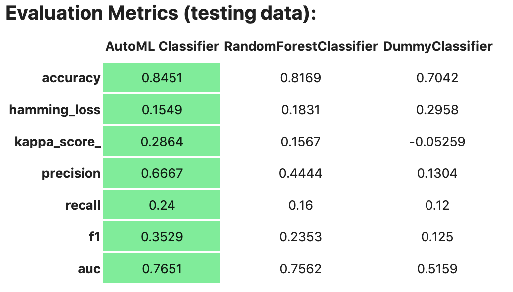
evaluator = ADSEvaluator(test, models=[model, baseline], training_data=train)
evaluator.show_in_notebook()
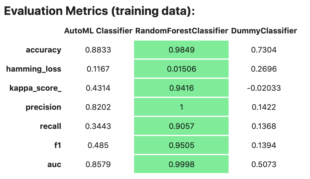
If you assign a value to the optional training_data method, ADS calculates how the models generalize by comparing the metrics on training with test datasets.
The evaluator has a property metrics, which can be used to access all of the calculated data. By default, in a notebook the evaluator.metrics outputs a table highlighting for each metric which model scores the best.
evaluator.metrics
If you have a binary classification, you can rank models by their calculated cost by using the calculate_cost() method.
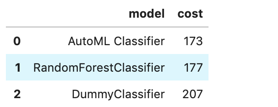
You can also add in your own custom metrics, see the Model Evaluation for more details.
Model Explanations
ADS provides a module called Machine learning explainability (MLX), which is the process of explaining and interpreting machine learning and deep learning models.
MLX can help machine learning developers to:
Better understand and interpret the model’s behavior. For example:
Which features does the model consider important?
What is the relationship between the feature values and the target predictions?
Debug and improve the quality of the model. For example:
Did the model learn something unexpected?
Does the model generalize or did it learn something specific to the train/validation/test datasets?
Increase confidence in deploying the model.
MLX can help end users of machine learning algorithms to:
Understand why the model has made a certain prediction. For example: - Why was my bank loan denied?
Some useful terms for MLX:
Explainability: The ability to explain the reasons behind a machine learning model’s prediction.
Global Explanations: Understand the behavior of a machine learning model as a whole.
Interpretability: The level at which a human can understand the explanation.
Local Explanations: Understand why the machine learning model made a single prediction.
Model-Agnostic Explanations: Explanations treat the machine learning model (and feature pre-processing) as a black-box, instead of using properties from the model to guide the explanation.
MLX provides interpretable model-agnostic local and global explanations.
How to get global explanations:
from ads.explanations.explainer import ADSExplainer
from ads.explanations.mlx_global_explainer import MLXGlobalExplainer

# our model explainer class
explainer = ADSExplainer(test, model)

# let's created a global explainer
global_explainer = explainer.global_explanation(provider=MLXGlobalExplainer())

# Generate the global feature importance explanation
importances = global_explainer.compute_feature_importance()
Visualize the top six features in a bar chart (the default).
# Visualize the top 6 features as a bar chart
importances.show_in_notebook(n_features=6)
Visualize the top five features in a detailed scatter plot:
# Visualize a detailed scatter plot
importances.show_in_notebook(n_features=5, mode='detailed')
Get the dictionary object that is used to generate the visualizations so that you can create your own:
# Get the dictionary object used to generate the visualizations
importances.get_global_explanation()
MLX can also do much more. For example, Partial Dependence Plots (PDP) and Individual Conditional Expectation explanations along with local explanations can provide insights into why a machine learning model made a specific prediction.
For more detailed examples and a thorough overview of MLX, see the MLX documentation.