Quick Start Guide

The Accelerated Data Science (ADS) SDK is a Oracle Cloud Infrastructure Data Science and Machine learning SDK that data scientists can use for the entire lifecycle of their workflows. You can also use Python methods in ADS to interact with the following Data Science resources:

• Models (saved in the model catalog)

• Notebook Sessions

• Projects

ADS is pre-installed in the notebook session environment of the Data Science service.

For a guide to ADS features, check out the overview. This Quick Start guide is a five minute compressed set of instructions about what you can accomplish with ADS and includes:

• Setting up ADS

• Getting Data into ADS

• Performing Data Visualization

• `Model Training with ADS`_

• Creating an ADSModel from Other Machine Learning Libraries

• Saving and Loading Models to the Model Catalog

• Model Evaluations with ADS

Setting up ADS

Inside Data Science Conda Environments

ADS is already installed in the environment.

Install in Your Local Environment

You can use pip to install ADS with python3 -m pip install oracle-ads.

Getting Started

import ads

Turn debug mode on or off with:

ads.set_debug_mode(bool)

Getting Data into ADS

Before you can use ADS for anything involving a dataset (visualization, transformations, or model training), you have to load your data. When ADS opens a dataset, you have the option to provide the name of the column to be the target variable during modeling. The type of this target determines what type of modeling to use (regression, binary, and multi-class classification, or time series forecasting).

There are several ways to turn data into an ADSDataset. The simplest way is to use ADSDataset or ADSDatasetWithTarget constructor, which takes as its first argument as a Pandas Dataframe object. The Pandas Dataframe supports loading data from many URL schemes, such as Object Storage or S3 files. The class documentation <https://docs.cloud.oracle.com/en-us/iaas/tools/ads-sdk/latest/modules.html>_ describes all classes.

For example:

• From a Pandas Dataframe instance:

import numpy as np
import pandas as pd
from sklearn.datasets import load_iris
data = load_iris()
df = pd.DataFrame(data.data, columns=data.feature_names)
df["species"] = data.target

from ads.dataset.dataset_with_target import ADSDatasetWithTarget

# these two are equivalent:
ds = ADSDatasetWithTarget(df, target="species")
# OR
ds = ADSDatasetWithTarget.from_dataframe(df, target="species")

The ds (ADSDataset) object is Pandas like. For example, you can use ds.head(). It’s an encapsulation of a Pandas Dataframe with immutability. Any attempt to modify the data yields a new copy-on-write of the ADSDataset.

Note

Creating an ADSDataset object involves more than simply reading data to memory. ADS also samples the dataset for visualization purposes, computes co-correlation of the columns in the dataset, and performs type discovery on the different columns in the dataset. That is why loading a dataset with ADSDataset can be slower than simply reading the same dataset with Pandas. In return, you get the added data visualizations and data profiling benefits of the ADSDataset object.

• To load data from a URL:

import pandas as pd

ds = pd.read_csv("oci://hosted-ds-datasets@hosted-ds-datasets/iris/dataset.csv", target="variety")

• To load data with ADS type discovery turned off:

import pandas as pd

pd.DataFrame({'c1':[1,2,3], 'target': ['yes', 'no', 'yes']}).to_csv('Users/ysz/data/sample.csv')

ds = ADSDatasetWithTarget(
  df=pd.read_csv('Users/ysz/data/sample.csv'),
  target='target',
  type_discovery=False, # turn off ADS type discovery
  types={'target': 'category'} # specify target type
)

Performing Data Visualization

ADS offers a smart visualization tool that automatically detects the type of your data columns and offers the best way to plot your data. You can also create custom visualizations with ADS by using your preferred plotting libraries and packages.

To get a quick overview of all the column types and how the column’s values are distributed:

ds.show_in_notebook()

To plot the target’s value distribution:

ds.target.show_in_notebook()

To plot a single column:

ds.plot("sepal.length").show_in_notebook(figsize=(4,4)) # figsize optional

To plot two columns against each other:

ds.plot(x="sepal.length", y="sepal.width").show_in_notebook()

You are not limited to the types of plots that ADS offers. You can also use other plotting libraries. Here’s an example using Seaborn. For more examples, see Data Visualization or the ads_data_visualizations notebook example in the notebook session environment.

import seaborn as sns
sns.set(style="ticks", color_codes=True)
sns.pairplot(df.dropna())

Creating an ADSModel from Other Machine Learning Libraries

You can promote models to ADS so that they too can be used in evaluations and explanations.

ADS provides a static method that promotes an estimator-like object to an ADSModel.

For example:

from xgboost import XGBClassifier
from ads.common.model import ADSModel

...

xgb_classifier = XGBClassifier()
xgb_classifier.fit(train.X, train.y)

ads_model = ADSModel.from_estimator(xgb_classifier)

Optionally, the from_estimator() method can provide a list of target classes. If the estimator provides a classes_ attribute, then this list is not needed.

You can also provide a scalar or iterable of objects implementing transform functions. For a more advanced use of this function, see the ads-example folder in the notebook session environment.

Saving and Loading Models to the Model Catalog

The getting-started.ipynb notebook, in the notebook session environment, helps you create the Oracle Cloud Infrastructure configuration file. You must set up this configuration file to access the model catalog or Oracle Cloud Infrastructure services, such as Object Storage, Functions, and Data Flow from the notebook environment.

This configuration file is also needed to run ADS. You must run the getting-started.ipynb notebook every time you launch a new notebook session. For more details, see Configuration and Model Catalog.

You can use ADS to save models built with ADS or generic models built outside of ADS to the model catalog. One way to save an ADSModel is:

from os import environ
from ads.common.model_export_util import prepare_generic_model
from joblib import dump
import os.path
import tempfile
tempfilepath = tempfile.mkdtemp()
dump(model, os.path.join(tempfilepath, 'model.onnx'))
model_artifact = prepare_generic_model(tempfilepath)
compartment_id = environ['NB_SESSION_COMPARTMENT_OCID']
project_id = environ["PROJECT_OCID"]

...

mc_model = model_artifact.save(
  project_id=project_id,
  compartment_id=compartment_id,
  display_name="random forest model on iris data",
  description="random forest model on iris data",
  training_script_path="model_catalog.ipynb",
  ignore_pending_changes=False)

ADS also provides easy wrappers for the model catalog REST APIs. By constructing a ModelCatalog object for a given compartment, you can list the models with the list_models() method:

from ads.catalog.model import ModelCatalog
from os import environ
mc = ModelCatalog(compartment_id=environ['NB_SESSION_COMPARTMENT_OCID'])
model_list = mc.list_models()

To load a model from the catalog, the model has to be fetched, extracted, and restored into memory so that it can be manipulated. You must specify a folder where the download would extract the files to:

import os
path_to_my_loaded_model = os.path.join('/', 'home', 'datascience', 'model')
mc.download_model(model_list[0].id, path_to_my_loaded_model, force_overwrite=True)

Then construct or reconstruct the ADSModel object with:

from ads.common.model_artifact import ModelArtifact
model_artifact = ModelArtifact(path_to_my_loaded_model)

There’s more details to interacting with the model catalog in Model Catalog.

Model Evaluations with ADS

Model Evaluations

ADS can evaluate a set of models by calculating and reporting a variety of task-specific metrics. The set of models must be heterogeneous and be based on the same test set.

The general format for model explanations (ADS or non-ADS models that have been promoted using the ADSModel.from_estimator function) is:

from ads.evaluations.evaluator import ADSEvaluator
from ads.common.data import MLData

evaluator = ADSEvaluator(test, models=[model, baseline], training_data=train)
evaluator.show_in_notebook()

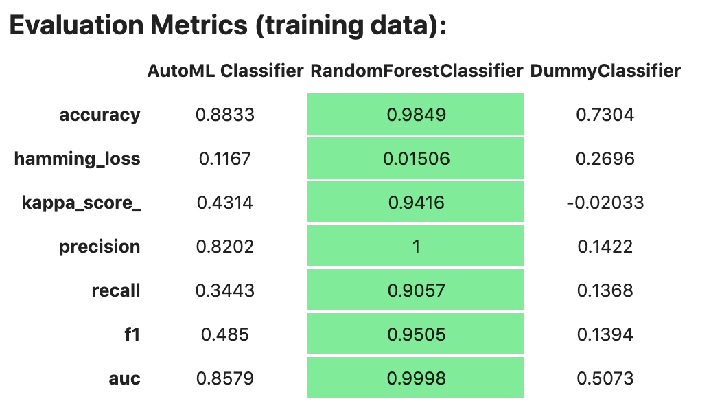
If you assign a value to the optional training_data method, ADS calculates how the models generalize by comparing the metrics on training with test datasets.

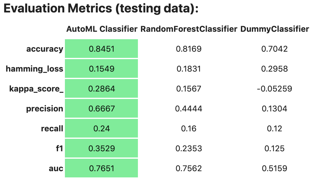
The evaluator has a property metrics, which can be used to access all of the calculated data. By default, in a notebook the evaluator.metrics outputs a table highlighting for each metric which model scores the best.

evaluator.metrics

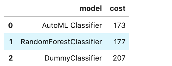
If you have a binary classification, you can rank models by their calculated cost by using the calculate_cost() method.

You can also add in your own custom metrics, see the Model Evaluation for more details.